SEC EDGAR API in Python#
by Michael T. Moen
The U.S. Securities and Exchange Commission (SEC) allows free public access to documents filed by publicly traded companies in the Electronic Data Gathering, Analysis, and Retrieval (EDGAR) system.
Please see the following resources for more information on API usage:
Documentation
Terms
Data Reuse
NOTE: Please see access details and rate limit requests for this API in the official documentation.
These recipe examples were tested on February 17, 2026.
Setup#
Import Libraries#
The following external libraries need to be installed into your environment to run the code examples in this tutorial:
We import the libraries used in this tutorial below:
from dotenv import load_dotenv
from math import log10
import matplotlib.pyplot as plt
import os
from pprint import pprint
import requests
Import User Agent#
An user agent is required to access the SEC EDGAR API.
We keep our user agent in a .env file and use the dotenv library to access it. If you would like to use this method, create a .env file and add the following line to it:
SEC_EDGAR_USER_AGENT="Institution, email@domain.com"
load_dotenv()
try:
    HEADERS = {'User-Agent': os.environ["SEC_EDGAR_USER_AGENT"]}
except KeyError:
    print("User-Agent not found. Please set 'SEC_EDGAR_USER_AGENT' in your .env file.")
SEC EDGAR Data Installation#
In addition to the publicly available API, SEC EDGAR data can also be access via a bulk data download, which is compiled nightly. This approach is advantageous when working with large datasets, since it does not require making many individual API calls. However, it requires about 15 GB of storage to install and is more difficult to keep up to date.
To access this data, download the companyfacts.zip file under the ‘Bulk data’ heading at the bottom of the SEC EDGAR documentation.
1. Obtaining Marketing Expenses for Amazon#
To access the data from an individual company, we must first obtain its Central Index Key (CIK) value. These values can be obtained by searching for a company here. Alternatively, you can find a list of all companies and their CIK value here.
For this section of the guide, we’ll use Amazon (AMZN) as an example, which has a CIK of 0001018724.
With this CIK, we can now build a URL for the /companyfacts/ endpoint:
BASE_URL = "https://data.sec.gov/api/xbrl/"
endpoint = "companyfacts/"
cik = "0001018724"  # CIK for Amazon

# Make the API request
response = requests.get(f"{BASE_URL}{endpoint}CIK{cik}.json", headers=HEADERS)

# Status code 200 indicates success
response.status_code
200
# Extract data from the response
data = response.json()

# Print the structure of the data
pprint(data, depth=2)
{'cik': 1018724,
 'entityName': 'AMAZON.COM, INC.',
 'facts': {'dei': {...}, 'us-gaap': {...}}}
# Explore some of the categories in the data
list(data["facts"]["us-gaap"].keys())[:10]
['AccountsPayable',
 'AccountsPayableCurrent',
 'AccountsReceivableNetCurrent',
 'AccruedLiabilities',
 'AccruedLiabilitiesCurrent',
 'AccruedLiabilitiesForUnredeeemedGiftCards',
 'AccumulatedDepreciationDepletionAndAmortizationPropertyPlantAndEquipment',
 'AccumulatedOtherComprehensiveIncomeLossAvailableForSaleSecuritiesAdjustmentNetOfTax',
 'AccumulatedOtherComprehensiveIncomeLossForeignCurrencyTranslationAdjustmentNetOfTax',
 'AccumulatedOtherComprehensiveIncomeLossNetOfTax']
We can also access individual pieces of information with our retrieved data:
NOTE: It may be useful to open the URL we created in Firefox, which has a built in JSON viewer that other browsers lack.
company_name = data["entityName"]
company_name
'AMAZON.COM, INC.'
For an example, let’s look at the yearly marketing expenses of Amazon, which is defined as “Expenditures for planning and executing the conception, pricing, promotion, and distribution of ideas, goods, and services. Costs of public relations and corporate promotions are typically considered to be marketing costs.”
# Navigate the JSON data structure to get us to the marketing expenses data
marketing_expenses = data["facts"]["us-gaap"]["MarketingExpense"]["units"]["USD"]

# Extract fiscal year and marketing expenses into a dictionary
yearly_marketing = {
    int(expense["start"][:4]): expense["val"]
    for expense in marketing_expenses
    if expense["form"] == "10-K"
}

# Display results
yearly_marketing
{2007: 344000000,
 2008: 482000000,
 2009: 680000000,
 2010: 1029000000,
 2011: 1630000000,
 2012: 2408000000,
 2013: 3133000000,
 2014: 4332000000,
 2015: 5254000000,
 2016: 7233000000,
 2017: 10069000000,
 2018: 13814000000,
 2019: 18878000000,
 2020: 22008000000,
 2021: 32551000000,
 2022: 42238000000,
 2023: 44370000000,
 2024: 43907000000,
 2025: 47129000000}
start_year = min(yearly_marketing.keys())
end_year = max(yearly_marketing.keys())
total_marketing_expenses = sum(yearly_marketing.values())

print(f"{start_year}-{end_year} total: ${total_marketing_expenses / 1e9:.2f} billion")
2007-2025 total: $301.49 billion
The following code block scales the data so that the y-axis of our graph contains smaller numbers that can be more easily understood, rather than large values in the billions.
# Break up the list of tuples forming 'yearly_expenses' into two separate lists
years, expenses = zip(*yearly_marketing.items())

# Create scale for bar graph
min = sorted(list(expenses), key=float)[0]
exponent = len(str(int(min)))

# Change the data to fit the scale
expenses = [x/(10**exponent) for x in expenses]
Finally, we can plot the data:
# Create graphing window with size 13x8
fig, ax = plt.subplots(figsize=(13,8))

# Format the bar graph
ax.spines["top"].set_visible(False)
ax.spines["right"].set_visible(False)
ax.spines["left"].set_visible(False)
ax.spines["bottom"].set_color("#CCCCCC")
ax.tick_params(bottom=False, left=False)
ax.set_axisbelow(True)
ax.yaxis.grid(True, color="#EEEEEE")
ax.xaxis.grid(False)

# Plot the graph and add titles
plt.bar(years, expenses, color="#4d4d4d")
plt.title(f"{company_name} Marketing Expenses")
plt.xlabel("Fiscal Year")
plt.ylabel(f"Marketing Expenses (* 10^-{exponent})")

ax.set_xticks(years)
ax.set_xticklabels([int(y) for y in years])

plt.show()
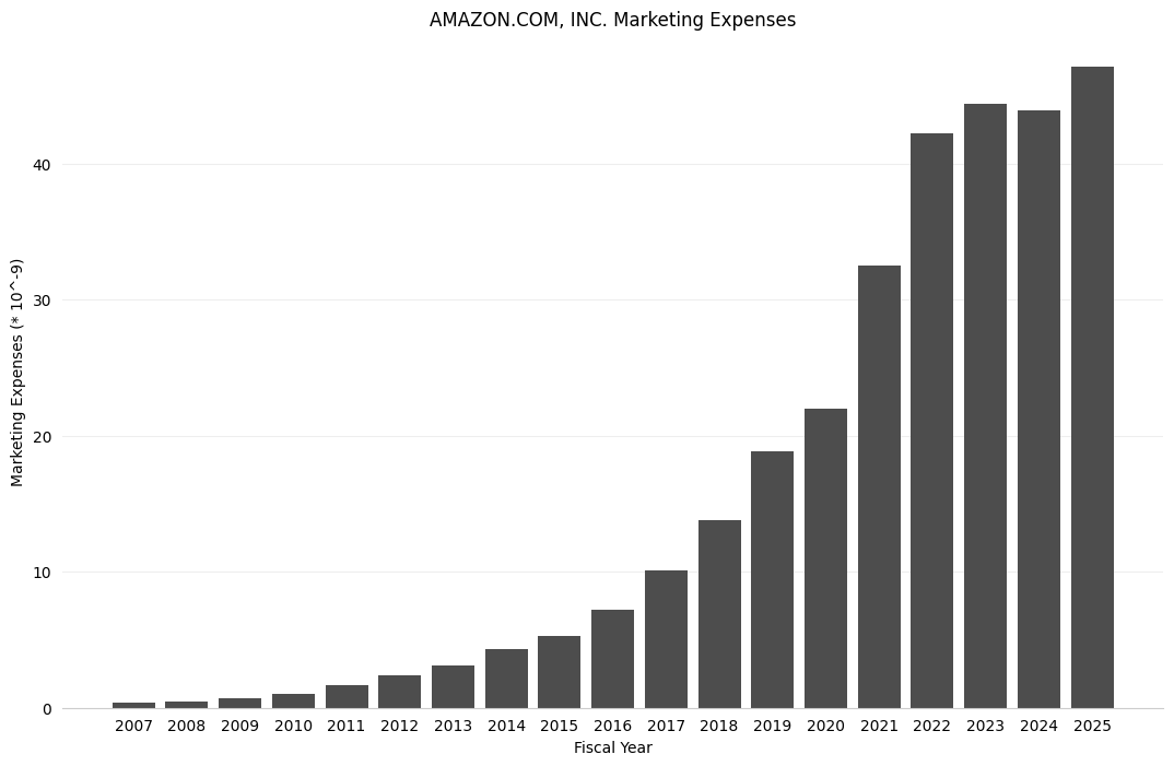
Note that the scaling of the data allowed us to present the data in terms of billions of dollars.
3. Comparing Total Assets of All Filing Companies#
The SEC EDGAR API also has an endpoint called /frames that returns the data from all companies for a given category and filing period. In this example, we’ll look at the total assets of all companies reported for Q1 2024.
# Categories can be found in the JSON data obtained from the /companyfacts/ endpoint
# Note that you also must include the units name for some categories (in this case, USD)
category = 'Assets/USD'
year = '2024'
quarter = '1'
url = f'https://data.sec.gov/api/xbrl/frames/us-gaap/{category}/CY{year}Q{quarter}I.json'

data = requests.get(url, headers=HEADERS).json()

# Display number of results
len(data['data'])
5838
Now, let’s retrieve the company names and asset values of all of the companies. Below, we store this data as a list of tuples in the total_assets list and sort it:
# Build list of tuples with (companyName, value) pairings
total_assets = [(entry['entityName'], int(entry['val'])) for entry in data['data']]

# Sort list of tuples by value of second part of tuple
total_assets = sorted(total_assets, key = lambda x: x[1], reverse=True)

# Display top 20 results
total_assets[:20]
[('FEDERAL NATIONAL MORTGAGE ASSOCIATION FANNIE MAE', 4323819000000),
 ('JPMorgan Chase & Co', 4090727000000),
 ('Federal Home Loan Mortgage Corporation', 3287373000000),
 ('Bank of America Corporation', 3273803000000),
 ('Citigroup\xa0Inc', 2432510000000),
 ('WELLS FARGO & COMPANY/MN', 1959153000000),
 ('The Goldman Sachs Group, Inc.', 1698440000000),
 ('MORGAN STANLEY', 1228503000000),
 ('BERKSHIRE HATHAWAY INC', 1070035000000),
 ('Prudential Financial, Inc.', 725823000000),
 ('US BANCORP \\DE\\', 683606000000),
 ('MetLife, Inc.', 677576000000),
 ('PNC Financial Services Group, Inc.', 566162000000),
 ('American International Group, Inc.', 544121000000),
 ('TRUIST FINANCIAL CORPORATION', 534959000000),
 ('AMAZON.COM, INC.', 530969000000),
 ('HDFC BANK LIMITED', 529380600000),
 ('MICROSOFT CORPORATION', 484275000000),
 ('CAPITAL\xa0ONE\xa0FINANCIAL\xa0CORP', 481720000000),
 ('SCHWAB CHARLES CORP', 468784000000)]
Graphing the Total Assets of All Companies#
Since the total assets of all companies is a dataset that ranges from values as low as zero to those as large as 4.3 trillion, these values must be graphed logarithmically. Below, we take the \(\log_{10}\) of each of the total asset values so that we can group the total assets in groups of ones (\(10^0\)), tens (\(10^1\)), hundreds (\(10^2\)), thousands (\(10^3\)), and so on. Then, we’ll use matplotlib to graph these values with a histogram.
Note: Since 0 is outside the domain of the log function, it must be handled separately in order to avoid throwing an error. In this case, we group these values into the ones (\(10^0\)) group, although this is not actually true.
# List of log10(total_assets) for each company
weighted_vals = [
    log10(company[1]) if company[1] > 0 else 0
    for company in total_assets
]

n_bins = int(max(weighted_vals)) + 1  # Number of bins to put data into for the histogram
bins = range(n_bins+1)                # Bin titles
# Create graphing window with size 13x8
fig, ax = plt.subplots(figsize=(13,8))

# Format the bar graph
ax.spines['top'].set_visible(False)
ax.spines['right'].set_visible(False)
ax.spines['left'].set_visible(False)
ax.spines['bottom'].set_color('#CCCCCC')
ax.tick_params(bottom=False, left=False)
ax.set_axisbelow(True)
ax.yaxis.grid(True, color='#DDDDDD')
ax.xaxis.grid(False)
ax.set_xticks(bins)

# Plot the graph and add titles
plt.hist(weighted_vals, color='#4d4d4d', bins=bins)
plt.title(f"Companies by Total Assets Reported for Q{quarter} {year} (Logarithmic)")
plt.xlabel("Assets (in 10^n USD)")
plt.ylabel(f"Number of Companies")

plt.show()
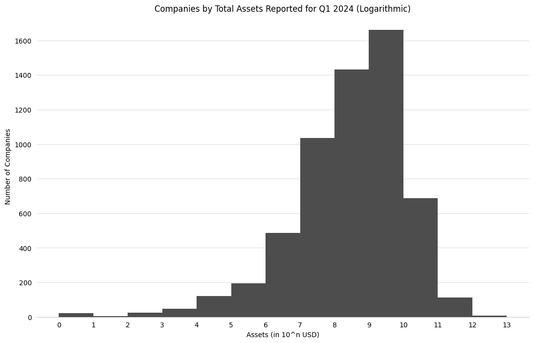
Note that for the above data, the 0-1 bucket indicates that a company reported between 0 and 9 USD in assets, while the 12-13 bucket indicates that a company reported between \(10^{12}\) and \(10^{13}\) (or one trillion and ten trillion) USD in assets.
4. Finding the Top 500 Companies by Revenue#
The Fortune 500 is a ranking of the top 500 companies by revenue, according to the data filed in their 10-K or a comparable form. In this example, we’ll look at only the revenues reported in the 10-K forms to construct a similar ranking of U.S. companies by revenue.
category = 'Revenues/USD'
year = '2024'
url = f'https://data.sec.gov/api/xbrl/frames/us-gaap/{category}/CY{year}.json'

data = requests.get(url, headers=HEADERS).json()

# Display number of results
len(data['data'])
2326
Now, we can sort this data by value and keep the top 500 results:
# List of tuples with ('company name', revenue) pairings
total_revenues = [(entry['entityName'], entry['val']) for entry in data['data']]

# Sort total_revenues by revenues
total_revenues = sorted(total_revenues, key = lambda x: x[1], reverse=True)

# Display top 20 results
for idx, company in enumerate(total_revenues[:20]):
    print(f'{idx+1:>3}. ${company[1] / 1e9:.2f}B: {company[0]}')
  1. $680.99B: WALMART INC.
  2. $400.28B: UnitedHealth Group Incorporated
  3. $372.81B: CVS HEALTH CORPORATION
  4. $371.43B: BERKSHIRE HATHAWAY INC
  5. $350.02B: Alphabet Inc.
  6. $349.58B: Exxon Mobil Corporation
  7. $293.96B: Cencora, Inc.
  8. $254.45B: COSTCO WHOLESALE CORP /NEW
  9. $247.12B: The Cigna Group
 10. $226.83B: Cardinal Health, Inc.
 11. $202.79B: Chevron Corp
 12. $187.44B: GENERAL MOTORS COMPANY
 13. $184.99B: Ford Motor Co
 14. $177.56B: JPMorgan Chase & Co
 15. $177.01B: ELEVANCE HEALTH, INC.
 16. $163.07B: Centene Corporation
 17. $137.30B: Alibaba Group Holding Limited
 18. $134.79B: Verizon Communications Inc.
 19. $130.50B: NVIDIA CORP
 20. $122.34B: AT&T INC.